Network Visualization
Using a *.txt file storing symmetric connectivity matrix and a *.csv table with nodal information (such as coordinate, label, module and color) as input, we can draw spheres and rods to visualize nodes and edges.
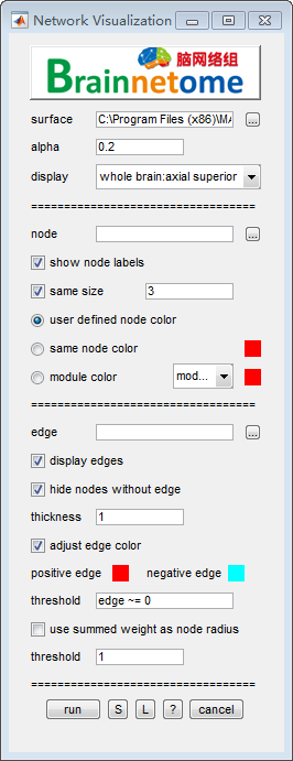
- surface: surface file
- alpha: degree of opaque
- display: mode of display
- node: node file defined as csv table. All columns are optional except for ‘x’, ‘y’ and ‘z’.
For example:
 x     y    z  size  module   r   g   b   label
 -1 , 20 , 20 , 4 , module1 , 5 , 5 , 5 , node1
-10 , 22 , 20 , 4 , module1 , 5 , 5 , 5 , node2
 12 , 20 , 20 , 4 , module2 , 5 , 5 , 5 , node3
- show node labels: check to show labels defined in input node file.
- same size: use same size for all node, uncheck to use user defined size in input node file.
- user defined node color: use color defined in input node file.
- same node color: use same color for all node.
- module color: use different color for each module. Modules are defined in input node file.
- edge: edge matrix for input file, the number of rows and columns should be the same as input file.
- display edges: display or not edges.
- hide node without edge: select not to show nodes without edge
- thickness: relative thickness for all edges
- adjust edge color: use different color for positive and negative edge.
- threshold: an expression that compatible with matlab syntax to filter out unwanted edges in edge matrix.
- use summed weight as node radius: sum up node’s degree and define node size.
- threshold: nodes with degree smaller than the threshold will not be shown.
- Buttons:
- S: Save parameters of the current panel to a
*.matfile. The*.matcan be further loaded for the panel or be used in a script processing. - L: Load parameters from
*.matfor the current panel. - ?: Help information.
- S: Save parameters of the current panel to a